We tested the captioning ability of 10 different vision-language models—models that can be prompted with both images and text and can output text in response*—in 1350 randomly selected head-to-head contests across 30 difficult-to-caption photographs. Below are the final rankings, by Bradley-Terry score. Click model cards for implementation details.
If you haven't been paying close attention to recent advances in computer vision, you may have missed vision-language models, which first appeared just a few years ago. Between 2012 and 2021, computer vision was dominated by convolutional neural nets trained on labeled data. In applied settings, this typically meant training or fine-tuning models on your own labeled data—assuming you had enough—or, alternatively, finding creative ways to use vector embeddings from interior layers of the network. That all changed in 2021, when OpenAI introduced CLIP (Contrastive Language-Image Pre-training). CLIP was trained with a contrastive loss on image/text pairs to align images and text in a shared embedding space. This was significant because it meant that you could now build a custom image classifier with no additional training: just embed your image and your target classes in the same vector space, and run k-NN on the class embeddings. More importantly, however, CLIP was a proof of concept for literate vision models and showed the vision transformer (ViT) to be the superior choice for encoding images. In short order, models began to appear that united literate image encoders (typically ViTs) with text decoders—i.e., large language models (LLMs). Now, models could not only see and read, they could also write. This innovation made captioning models possible, and these are the subjects of the present study.
Overall Rankings
-
gpt-4o-2024-08-06 0.213
-
gemini-1.5-pro 0.133
GPU requirements unknown
Precision unknown
3072px max (our images are only 2048px), tiling unknown
$0.03
-
claude-3-5-sonnet-20241022 0.122
GPU requirements unknown
Precision unknown
1568px max, tiling unknown
$0.22
-
allenai/Molmo-72B-0924 0.115
-
Qwen/Qwen2-VL-72B-Instruct 0.114
-
OpenGVLab/InternVL2-Llama3-76B 0.077
-
nvidia/NVLM-D-72B 0.072
-
lmms-lab/llava-onevision-qwen2-72b-ov 0.058
-
rhymes-ai/Aria 0.055
-
llama-v3p2-90b-vision-instruct 0.041
Methods
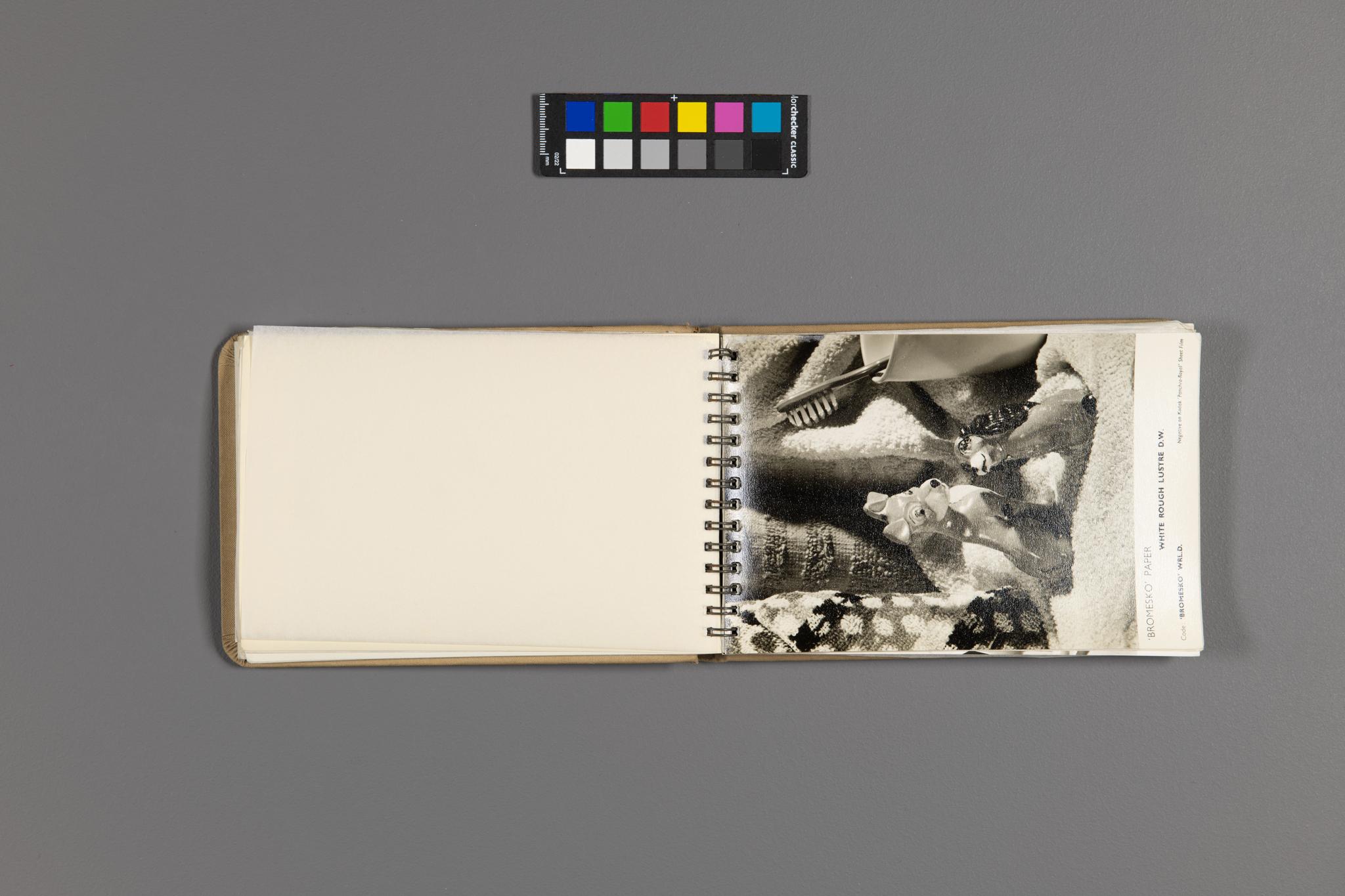
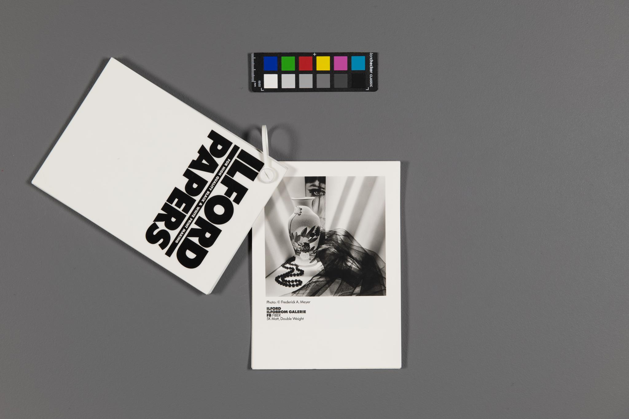
We selected 30 photographs from our collection of historic photographic sample books to test the image captioning abilities of 10 of today's biggest vision-language models (VLMs). The photos were chosen primarily for their difficulty [Fig. 1]. Each photo is shown embedded in the pages of a photographic sample book, which is itself sitting on a grey background beneath a color checker. The models therefore need to find the photo before captioning it, and although we write our prompt with this in mind, models struggle to ignore this irrelevant visual context.
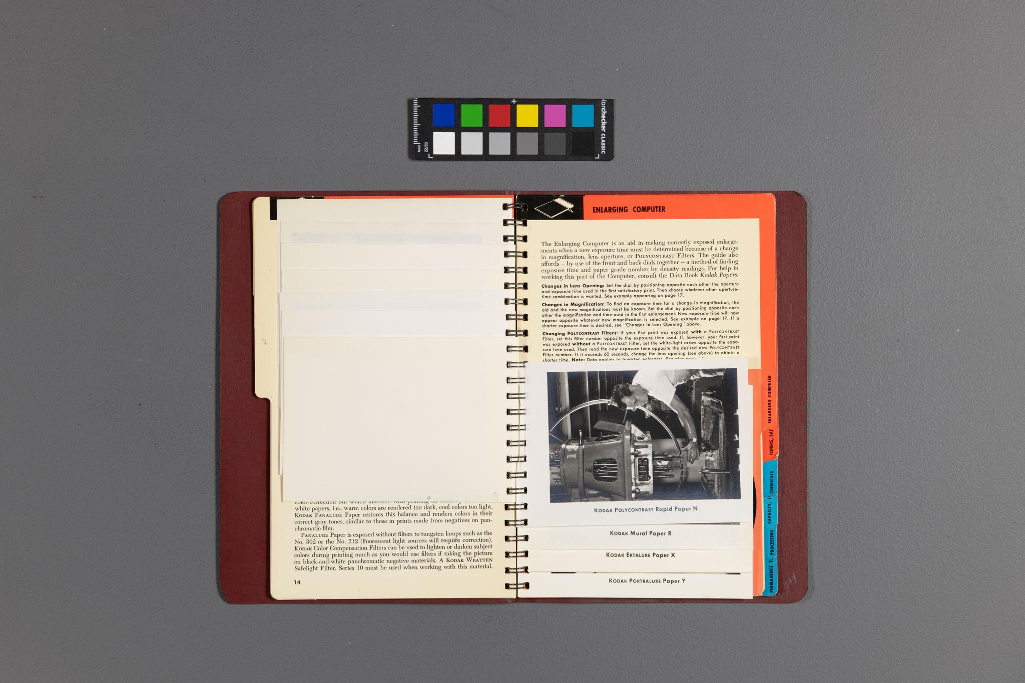
Our sample books are always imaged in an upright orientation. But in some cases, the photographs within are mounted sideways, and we did not correct for this before passing these images to the models. Some photos are damaged, some are pictured on pages together with lots of irrelevant text, some of the photos are very small, and many have visual content that is ambiguous or otherwise difficult to parse. This made it easier to choose between competing models, because many performed poorly in these conditions.
We used the following prompt:
There are two objects in this image. One is a color checker, and the other is a photographic sample book, open to a page containing a photograph. Give a detailed description of the photograph.
Slight variations of this prompt were used in certain cases, depending on where the model authors recommended putting a special image token (sometimes before the prompt, sometimes within it).
We started by obtaining 300 image captions, one from each of 10 models for each of 30 images. Each model was inferenced only once for each image; we did not, for example, choose among several outputs for the same prompt. The closed models—GPT-4o, Gemini 1.5 Pro, and Claude Sonnet 3.5—were inferenced via API, using the standard API examples with default settings (apart from max output tokens, which was always set to 1024). Llama 3.2 was inferenced using the Fireworks API. All other open models were inferenced using the code provided in their Huggingface repos, with default settings. Click model cards in the above section for links to our actual inference code. Open models (apart from Llama) were inferenced using cloud GPUs on Jarvis Labs, inside their JupyterLab servers. These models are large, and typically needed 4 GPUs, each with 48GB VRAM (I used A6000s).
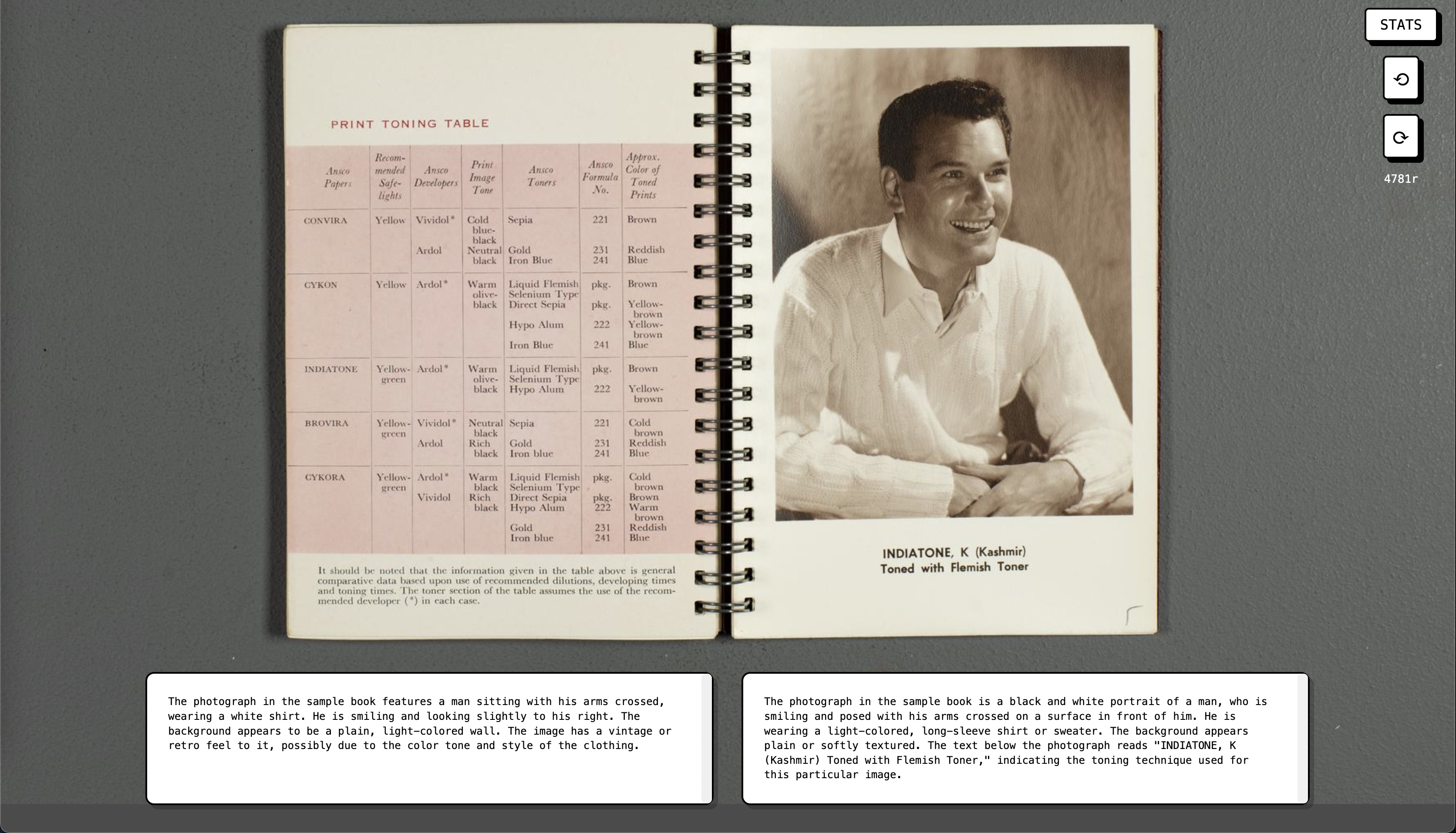
Once we obtained the captions, we built a web tool that displays an image and a pair of captions, both randomly selected and without any identifying information [Fig. 2]. Human judges were instructed simply to choose the better caption. We did not provide any further instruction, so judges were not likely using the same selection criteria. We did, however, avoid the worst forms of open-ended evaluation (like bad faith participation in a public evaluation platform) by strictly controlling court appointments: all judges are members of our lab and are experts in the material history of photography. There were 5 human judges, though judgments were not evenly distributed across them. We collected 1350 judgments in total, because this is the number you'd need for every image to see every model pairing. Because the contests were chosen at random, it is not the case that every image saw every model pairing.
After judging 1350 contests, we ran Bradley-Terry scoring on the results and obtained the ranking above.* Bradley-Terry is a scoring algorithm that takes pairwise comparisons as input and uses maximum likelihood estimation to assign scores (strengths) that explain these comparisons. It answers the question what strength each competitor would need to have to explain the totality of contest outcomes. Bradley-Terry models these strengths as follows:
$$P(A \text{ beats } B) = \frac{\text{strength}(A)}{\text{strength}(A) + \text{strength}(B)}$$
Because it makes sense to view our contest data as a sample drawn from a much larger universe of potential contests, our Bradley-Terry scores are only estimates of the true
model strengths. Accordingly, we need to quantify the uncertainty in these estimates. Bradley-Terry scores are estimated from 1000 bootstrapped samples of the contest data [notebook]. And because our contests are not entirely independent of one another—their outcomes depend in part on the images being captioned—we need also to account for this additional source of variability in our resampling procedure. We begin by grouping contests by image. Then, for each iteration of the bootstrap, we select a sample of groups and build a contest set by adding all contests from each group. Bradley-Terry scoring is computed on the contest set, and after 1000 iterations, we have 1000 sets of Bradley-Terry scores. The scores reported in the table above are the mean values across these 1000 sets. The bootstrap procedure also makes it easy to obtain confidence intervals around score estimates: the bounds of a 95% confidence interval around each score are the values of its 2.5 and 97.5 percentiles, respectively. Assuming that our raw contest data is broadly representative of the universe of all possible contests, this means that if our entire study were rerun many times, 95% of the intervals computed in this way would include the true score for each model.
Observations
In the course of making model comparisons, we also made a number of observations about model behavior in this unique competition environment. Below is a selection of some of the more interesting observations, organized into two subsections highlighting, in turn, quantitative and qualitative characteristics of model behavior.
Quantitative Observations
Ranking Stability
GPT-4o is the clear winner by a large margin. It took the top spot in the Bradley-Terry rankings after only 18 contests—despite competing in only 4 of them!—and never left that spot again. The final rankings were more or less in place after 125 contests—less than 10% of the total—with only slight variations thereafter.
Performance Overlap
It should be pointed out, however, that because Bradley-Terry models pairwise win probabilities, we can interpret model scores pretty directly, and the mere fact of their stability does not imply that the rankings capture extreme differences in performance. There is, to be sure, a gulf between the best and worst models: the probability of the best model (GPT-4o) beating the worst (Llama) is:
$$\frac{0.214}{0.214 + 0.041} = 0.84$$
That is, GPT-4o would beat Llama 84% of the time, according to our human judges. However, local differences are far less impressive: the probability of the best model (GPT-4o) beating the second best (Gemini) is only:
$$\frac{0.214}{0.214 + 0.131} = 0.62$$
This means that, in well over a third of head-to-head contests between GPT-4o and Gemini, Gemini would win. In the group of 4 models ranked immediately below GPT-4o, most contests are essentially a toss-up.
Open Source Performance
This is of particular interest because two of those four essentially equivalent models are open source! Although the top three spots went to closed models, the story of the rankings is not closed models, then everything else
. Molmo and Qwen are much closer to Gemini and Claude than they are to the rest of the pack, and much closer than those closed models are to GPT-4o. GPT-4o is in a class of its own, and Molmo and Qwen are in the same class as Gemini and Claude. That's the headline. Of course, all model authors will say this about their models and ground the claim in cherry-picked benchmarks, but this is a field study
and cannot be gamed.
It's also worth pointing out that, despite its low rank in this study, Aria is a remarkable achievement. Its performance was statistically indistinguishable from both Llava and Llama, despite needing half the VRAM and ~10% of the cost. Moreover, Aria's decoder is trained from scratch! It's possible there are other smaller models that can compete in this range, but Aria was the only size outlier in this study.
Cost
That said, apart from having executive control over the weights and perhaps dodging certain security concerns, it's not altogether clear that you're better off using an open model. Certainly, I believe in the ethos of open software. But in this case, the closed models are far cheaper because you're only paying for the inferences, not the time it takes to download the model and load its weights into VRAM. And even ignoring the initialization cost, consumer GPU rental is simply more expensive than API use on a cost-per-inference basis. Gemini in particular is extraordinarily cheap. Consider that, to get 30 inferences, Gemini cost just $0.03 while Molmo cost $27.
Image Resolution
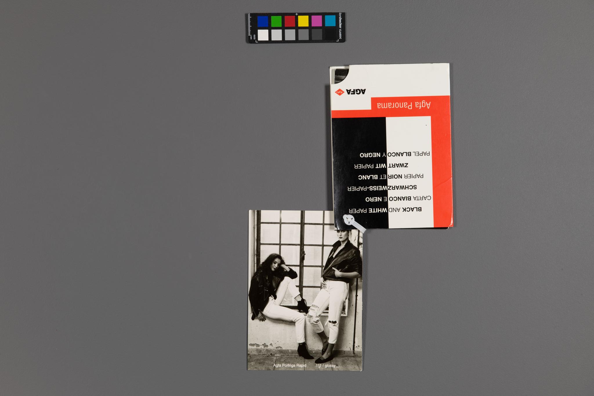
Early VLMs (2021-2023) tended to use fixed input resolutions, and often, these resolutions were quite small: 336px in the original version of CLIP, for example. More recently, dynamic tiling was introduced [UReader] [InternVL] as a way to capture a greater share of an image's native resolution. Models will generally place limits on the number of tiles—and very large images are downsampled before tiling—but images of the size used here (2048px on the long edge) are submitted in close to their native resolutions across most of the models in the study. We can't know for sure what the closed models are doing (although OpenAI is somewhat more transparent than the other labs), but we do know that all but two of the closed models use some form of tiling. The two that do not are Aria and Llama, the two worst overall performers in our study. This is not, of course, conclusive evidence that input resolution is playing a direct causal role in model performance, but there's a fairly plausible information-theoretic argument for such a role, and a model that downsamples an image whose relevant content is already only a fraction of the total image resolution is likely to have problems resolving this content [Fig. 3]. Because of this, it appears that VLM teams are making the right decision to use dynamic tiling.

Qualitative Observations
Spatial Relations
Dynamic tiling is a bit of a no-brainer in any case, because vision transformers (even pre-tiling) have always split image inputs into patches prior to the encoding step. The two methods have similar structure: an image (or tile) is split into non-overlapping squares and made sequential before reaching the attention blocks. The original sequence positions of the patches or tiles are typically tracked—via position embeddings, common to all transformers—in order to preserve important relational information between them. Without position embeddings, the vision transformer would be operating on a bag of patches
representation and unable to perceive spatial relations in images. The VLMs studied here tend to do well with spatial relations, although spatial ability is a clear differentiator in some cases.
One initially puzzling case arises in the distinction between allocentric and egocentric spatial coordinates: models are generally good at the former—at saying, for example, that some object appears on the right or left side of the image—but only the best models are able accurately to assign right
and left
to a person's arms. If an image portrays a person facing the viewer, her right arm will appear on the left side of the screen, and most VLMs struggle to translate this allocentric location into egocentric coordinates [Fig. 4]. Somewhat amusingly, they will try nonetheless!
...The woman on the left is seated, her legs crossed, and she props her right arm on her raised knee...The woman on the right stands with her left knee slightly bent, one hand on her hip, and the other supporting herself against the window frame...
The model is trying to navigate the spatial complexity of the scene, and clearly has been trained to make reference to the egocentric frame—right armand
left knee—but is getting it wrong, despite (or perhaps because of?) excellent performance in the allocentric frame.
But even within the allocentric frame, there are challenges that separate wheat and chaff, and none so potentially disruptive to captioning performance as nonstandard rotational orientation. In our study set, 9 of the 30 photos are pictured sideways, and only the very best models were able to translate from the sideways to the upright frame. The difficulty here is structurally similar to the problem of egocentric coordinates: the model's position embedding is correctly describing the scene on a particular assumption about the reference frame, but the assumption is false. In both cases, the position embedding itself is not to blame, but rather the learned relationship between certain position-embedded sequences and the corresponding scene content. The fix, then, is likely in the training data and not the architecture. To be sure, models can differ in their position embedding architectures*, but these differences do not explain the performance gaps we see here. And how could they? No amount of accurate position tracking can teach the model that limbs are named in the egocentric frame, or that certain spatial arrangements of objects are so unlikely as to recommend a reorientation of the input image. That's not an encoding issue; it's a knowledge issue, and you solve knowledge issues with better training data.
One perhaps surprising fact about position embeddings in vision transformers is that they do not—with the exception of Qwen—explicitly encode 2D position. Such encodings have been tried but have been shown to confer no performance advantage over 1D embeddings [ViT], and in some cases [NVLM], 2D embeddings are reported to perform worse! It's unclear why this should be—apart from, perhaps, being harder to train effectively—but we do know why 2D position embeddings are typically not necessary: 1D position embeddings are absolute, meaning that they are indexed to specific locations in an image. Provided that your input size is fixed, position 17—to use an imagined example—will always refer to the same region of any image encoded by the network. Importantly, position 17 will always be below position 5, to the right of position 13, etc.
Early VLMs used fixed-size, single-image inputs, and modern VLMs typically use dynamic-resolution inputs with fixed-size tiles. In our study—ignoring the closed models, which we know little about—the only exception to this design is Qwen, which uses variable-size inputs without tiling, and thus cannot use absolute position embeddings. Instead, it uses rotary position embeddings [RoPE], which encode both absolute and relative position information, making it possible to track spatial relations across images of different sizes.
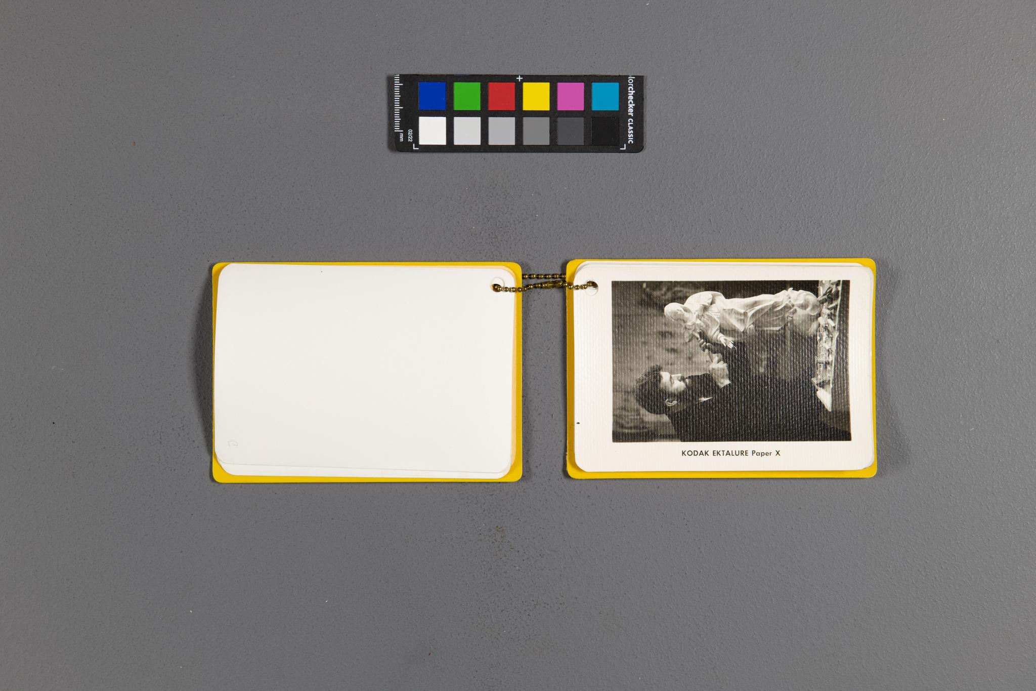
The photograph depicted in the image is a black and white portrait of a middle-aged man lifting a child above his head...
Or similarly, from Qwen:The photograph depicts a scene with two indiviudals. One person is lying down, possibly on a bed or similar surface, while another person is standing over them...
These behaviors point up the extent to which models are engaging in sensemaking, rather than simply reporting the identities of and relations between atomic scene elements.It's instructive to observe how models adapt in these situations. A model will rarely respond that a scene is confusing or hard to parse; it will make an attempt no matter the conditions. From this observation, we learn that models are not reporting faithfully on what they see (or don't see); rather, they are telling whichever coherent story is most probable, given the weak visual guidance they are receiving. A standing tree in a sideways photo becomes a fallen tree
; a rotated scene of a sculptor and his work becomes a man lifting a child above his head
[Fig. 5]; and an unusual scene involving two dog figurines, a terry cloth towel, and a toothbrush [Fig. 6] becomes, when seen on its side, the stage for an eclectic revue of confabulations you'll have to witness with your own eyes in the Appendix.
Varieties of Inductive Bias
This amusing behavior likely stems from the fact that we human judges see only the output of the VLM's text decoder, and this output is underconstrained by the VLM's vision encoder. A typical VLM unites a vision transformer [ViT]—the encoder, or the thing that sees—with a large language model (LLM)—the decoder, the thing that writes. Because all model outputs are authored by the decoder, we have only indirect access to its visual encodings. My hypothesis is that, in the handful of cases where our models truly struggle, the relevant visual encodings are themselves very weak, because the ViT's attention heads simply don't know what to focus on: nothing they saw during training prepared them for such cases.
But why should it be so difficult to read these cases? To be sure, the sideways orientation of dog-dog-towel-toothbrush makes an already unusual scene even harder to parse. But there are upright examples that caused similar difficulty [Fig. 7]. What unites these cases, it seems, is that they are all non-natural scenes containing unlikely juxtapositions of objects. The objects themselves needn't be difficult to identify on their own; what matters is that their co-occurrence is tough to interpret in a globally coherent way. And this reveals a structural weakness of ViTs: because they use global self-attention to encode visual inputs, their apprehension of these inputs is biased in favor of global coherence, which can be absent in non-natural images.
It is commonly said that vision transformers have weak inductive biases because they lack the hardwiring for locality and translation equivariance we see in convolutional neural nets (CNNs). This much is true, and indeed, CNNs are less likely to struggle with the cases at issue here, because, provided they can suitably represent the atoms—a dog figurine, a towel, a toothbrush, etc.—they will not be confounded by unusual arrangements of these atoms. If a CNN can recognize an object in one position, it can recognize it in any position, because the relevant filter weights are shared at every location in the image.
But vision transformers have their own inductive biases. Because self-attention on pixels is computationally infeasible even at normal image resolutions, ViTs operate on image patches. This means that ViTs can localize features at the patch level and not any lower. Moreover, patches do not overlap, and it will often be the case that objects of interest cross patch boundaries, making their recognition more difficult. But more importantly, I argue that (global) self-attention in ViTs itself introduces a kind of inductive bias. This is controversial: in self-attention, every element (here, an image patch) attends
to every other element in the sequence. This enables transformers to track long-range dependencies, which is crucial in language modeling, where such dependencies are common. Importantly, self-attention does not enforce the modeling of long-range dependencies; it only makes them as modelable as short-range dependencies. It is range-neutral in this respect, and thus does not count as an instance of bias—or so the argument goes. I disagree.
In language, both short- and long-range dependencies are common, and thus treating them (in the wiring) as equally important might very well count as neutral. But in images, long-range dependencies are not common; at least, they are not nearly as common as short-range ones, and this is especially true for the images at issue here. Because of this, attention scores for a wide range of image inputs are comparatively weak, because they contain no long-range dependencies. This has downstream effects on induction. In particular, as I am hypothesizing here, these weak attention scores, when passed to a decoder, leave unfilled the inferential role that global coherence would normally fill in a text sequence. Without it, the decoder is vulnerable to the gravity of its own learned attractors, and instead of talking directly about its visual inputs, it will tell whatever coherent story it can reach from this weak starting point, like a student stumped by an exam question, trying to earn points by demonstrating knowledge about something nearby or venturing a reasonable guess, given the little that she does remember [Fig. 8].

The photograph in the open sample book shows the iconic Trevi Fountain in Rome, Italy. This famous Baroque masterpiece is captured in all its grandeur, with its elaborate sculptural elements and cascading water...The Trevi Fountain's central feature - a large seahorse-drawn chariot - is likely visible, though details may be somewhat obscured due to the nature of the photograph. The fountain's ornate architecture and the play of light on the water create a captivating visual composition. This photograph beautifully captures one of Rome's most beloved landmarks, showcasing its architectural splendor and the enchanting atmosphere it creates in the heart of the city.
The model, trapped deep in the grooves of the Trevi hypothesis, even gins up an explanation for why some of its distinctive features are missing. This is a clear case of a model underconstrained by its visual inputs, warped out of balance by the overrepresentation in its training data of one particular set of related features.And in fact, the situation is likely even worse than it would seem when considering self-attention on its own. For, self-attention interacts with the other forms of bias: what counts as a local or short-range relationship in patched
self-attention will depend on the semantics of patches, and this in turn depends on their size and on the field of view of the input image. Do patches contain objects? Parts of objects? Parts of objects are likely related; whole objects may not be. It's very possible in the unlucky cases that, despite counting as well-formed
and physically coherent, an image may lack both long- and short range dependencies on the definition implied by self-attention and the model's particular patching schedule. So despite containing substantive content, an image is seen by the model the way a vague, meandering sentence might be seen: entirely lacking semantic direction. Or, in case the patching finds suitable alignment with the image's composition and scale, the image might thereby present the opposite shortcoming: semantic vectors pointing in every direction, too numerous to reconcile, averaging to nothing.
To put the point more concretely: consider that the correct caption for any particular hodgepodge of items is unlikely to appear in any training dataset. So how, then, is the decoder supposed to generate this caption? Weak attention scores from the ViT provide insufficient visual guidance, and the decoder cannot fill the gaps by adverting to relationships it has learned during training: no such relationships appeared during training, and in a sense, no such relationships exist even here, in the input image. Items appearing together in an image needn't stand in any semantic relationship at all, and this makes images quite unlike text sequences, where this sort of disjunction of semantic atoms is extremely uncommon. In fact, the only place it is likely to appear is, indeed, as a description of a visual scene, and there simply aren't enough such descriptions living in the open internet to make hodgepodge captioning possible for any but the very deepest of data scrapes (or, alternatively, the cleverest of data synthesizers). When you remove all image-focused hardwiring from a network, enforce a semantically blind individuation regime on its inputs, and make pairwise relations between these semantically noisy atoms the precondition for inferential power, you get disappointing results for any case lacking a critical mass of textural counterparts in your training corpus.
Looking Ahead
We've here focused primarily on the ways in which hostile conditions can act as a differentiator, but in truth, the default mode for modern VLMs is convergence. The models in our study perform similarly in the ordinary cases, and sometimes quite similarly. Compare these two captions:
The photograph in the sample book shows a young child standing and smiling. The child is wearing a short-sleeved shirt, shorts, and oversized shoes that appear to be too big for their feet...
---
The photograph in the sample book shows a young child standing and smiling. The child is wearing a short-sleeved button-up shirt, shorts, and large shoes that appear to be oversized for them...
The top caption is from Llava, the bottom from Aria. This degree of overlap might be expected from two VLMs using the same text decoder (as is common in this study), but that's not the case here: Aria is trained from scratch! Clearly, a great deal of shared training data is to blame. And in this case, the sharing is innocuous (or even beneficial), because the captions are good. But we've also described a number of shared failure modes, if they rest on the sharing of incomplete or otherwise suboptimal training datasets, here is a clear opportunity to improve.
We've seen some hints. For one, augmenting whatever we've already got with rotations and translations could go a long way to making the encoding of spatial relations less brittle. We might also prune redundant scenes from our training data, because they overweight the model in favor of certain sets of related features. Additionally, it's pretty clear that there are data gaps in the hodgepodge
image genre, as you might expect: it's a tough genre to span, because its defining feature is heterogeneity. Assuming an encoding architecture—like the ViT—that needs to learn all regularities from data, it's likely that there simply isn't enough naturally occurring image data to fill the gaps. This is where synthetic data comes in, and we see pretty clear evidence that models are already using it: the InternVL captions are lousy with markdown hashes and stars, for example. Clearly, the training data being reconstructed in these captions did not originate in human annotators. A good sign, but plenty more work to be done there.
It might be suggested, additionally, that architectural modifications could relieve some of the burden that currently rests on training data. Biases designed specifically for images could solve some of our problems here without additional data; indeed, there are already several attempts in the literature to add CNN-style hardwiring to ViTs [Swin Transformer] [CvT]. But custom architectures can be fiddly and difficult to scale, and it's more likely that the simplest architectures—pure transformers—will ultimately win out, with necessary improvements made entirely on the data side. This may have happened already, of course, in closed models like GPT-4o, and if so, it's only a matter of time before open models catch up.
Appendix
In this appendix, we include all 10 captions for all 30 images. Navigate left and right using either the arrow keys on your keyboard or the white arrow buttons to the left and right of the image. The captions are ordered by Bradley-Terry strength. Click on a model card to see the caption. The images are presented exactly as the models saw them, so if a photograph is rotated, that means the models saw the rotated version.